Neighbor-Aware Vision Transformer

A plastering robot has to answer one question before it moves its arm: should I put material here, smooth what is already on the wall, or leave this part alone. It answers by looking, and the looking was my master's thesis at the Kyoto Institute of Technology.

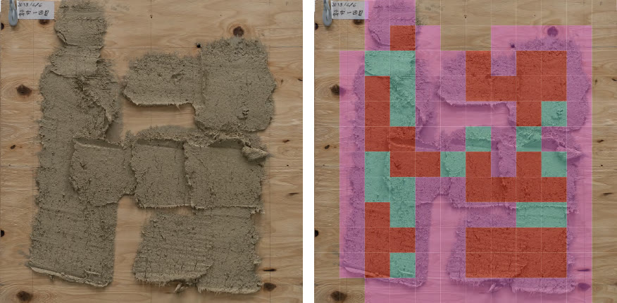
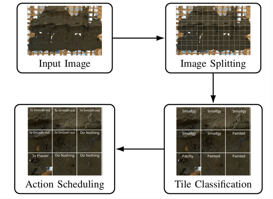
The system takes one high-resolution photograph of a wall, cuts it into about a hundred and forty square tiles, and sorts each tile into one of four surface states. Painted means the tile is finished. Patchy means material is there and does not cover. Smudgy means it covers and sits unevenly. Unpainted means bare wood. Those four states map onto three commands, plaster, smooth, or ignore, and the whole wall comes back as a CSV of tile coordinates that the robotics team feeds to their arm.

The reason anyone wants this is that Japanese plastering is done with a trowel and natural mud by people who are getting harder to find, and a robot that takes some of the work has to see the wall the way a plasterer sees it. The work became an IEEE paper I presented in Xi'an as first author.

A mud-plastered wooden wall photographed straight on, and beside it the same wall covered in a grid of colored tiles marking each patch as painted, patchy or smudgy. — One wall in, one grid of commands out. Red is painted, green is smudgy, pink is patchy.

The model only knew one wall

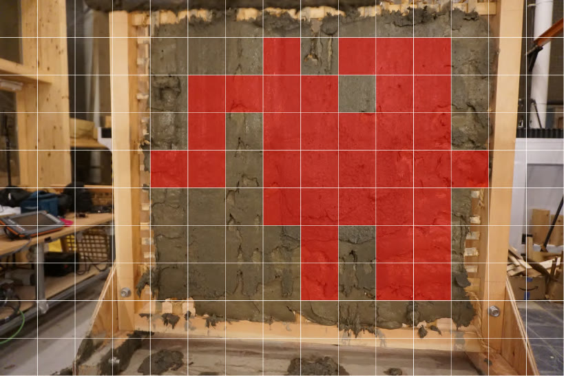
The lab already had a classifier when I arrived, a VGG16 that labeled each tile painted or not painted. It had been trained on photographs of a single wall type with a single paint texture, and on that wall it worked. The figure below is that model shown a wall it had never seen, a bamboo lath frame covered in mud, and the tiles it calls painted are scattered across it in a pattern that does not correspond to anything on the wall.

Binary labels were also too coarse for the job. "Needs plastering" covers bare wood, a zone where the mud went on too thin, and a coat that is thick enough but ridged, and those three want three different movements from the arm. So I relabeled the problem into four states chosen for what the robot should do about them, which is why the classes are named the way they are.

A mud-covered bamboo lath wall with a grid overlay, where scattered tiles are shaded red by the old binary model. — The previous model on an unfamiliar wall. Red tiles are the ones it called painted.

Four states, and what the tiles said about each other

The university had about three hundred wall photographs. I took forty-two of them, picked for how much they differed from each other in lighting, wall material, paint type and camera angle, because I wanted the model to hold up on walls it had not seen and I had six months rather than a year of data collection. Each image splits into roughly a hundred and forty-four tiles, which gave 5,952 tiles for training and validation. Twelve further images stayed out of all of it and produced 1,696 test tiles.

I annotated every one of those tiles myself, around five minutes per full image. That is also the dataset's weak point and I would raise it first if someone asked: one annotator means no inter-annotator agreement, and the boundary between a light smudge and a finished surface is genuinely arguable, so some of the fold-to-fold variability further down is probably mine.

Then I counted. For each class I took every tile of that class and tallied the classes of its eight neighbors. Around unpainted tiles almost every neighbor is unpainted or patchy. Painted sitting directly next to unpainted is close to absent from the dataset. Surface states come in runs, because a person plastering a wall works in strokes, and a tile of wet mud and a tile of shadow that look alike on their own stop looking alike once you can see what surrounds them.

Four panels: the input wall photograph, the same image split into a grid, each tile labeled smudgy, painted or patchy, and the same grid turned into robot actions. — Input image, tiles, one of four states per tile, then the command the arm receives.

Nine tiles through the same encoder

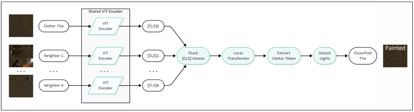
So the model reads a 3×3 window, the tile being classified and the eight around it. All nine go through the same Vision Transformer encoder with shared weights, which means the model learns one notion of what plaster looks like instead of nine. The nine resulting tokens are stacked and passed through a small transformer that lets them attend to each other, and then only the center token goes to the classification head. The neighbors are there as context and never receive a prediction of their own.

At the edges of an image a neighbor is missing, and I fill it with a black tile. That is a blunt choice and it can teach the model something about borders that has nothing to do with plaster, which is written into the paper as a limitation rather than left for someone to find.

I ran the obvious variations on the context module. One transformer layer gives a macro-F1 of 0.8014, a lighter encoder 0.8116, three stacked layers 0.8208, and three layers with the lighter encoder 0.8283. The ablation is thin, nine identical encoders in parallel is the straightforward design and not the efficient one, and both of those are in the report as work for whoever comes next.

Diagram of the Neighbor-ViT pipeline: center tile and eight neighbors each entering a shared ViT encoder, their tokens stacked, a local transformer, center token extraction, output logits, one classified tile. — Nine tiles in, one classified tile out. The encoder is the same block nine times over.

Five models, one protocol

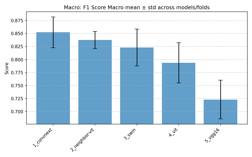
When I submitted the paper I had benchmarked against two baselines, VGG16 and a plain ViT, and the paper reports that run. Afterwards I added ConvNeXt and Swin Transformer and re-ran all five under the same training protocol and the same five-fold split, which is the comparison below.

ConvNeXt has the best mean macro-F1 at 0.852. Mine is second at 0.838. The column I care about is the spread across folds: 0.017 for the neighbor-aware model against 0.030 for ConvNeXt and 0.039 for a plain ViT. With forty-two images the folds are heterogeneous, so a model that moves less between them is telling you something about how it will behave on a wall nobody photographed, and for an arm that has to act the same way twice that mattered more to me than the third decimal of a mean.

The price is inference time. A batch of sixteen takes 0.132 seconds against 0.023 for a plain ViT, because nine encoder passes happen where there used to be one. On this dataset that is a fair trade, and on a wall where the arm has to keep up with a person it might not be.

Bar chart of macro-F1 across five models with error bars: ConvNeXt highest with a wide bar, neighbor-ViT second with the narrowest, then Swin, ViT and VGG16. — Macro-F1, mean and standard deviation over five folds. The error bars are the point.

What the lab kept

My deliverable was the vision side: the camera logic, the model, the training pipeline, and the CSV of per-tile commands. The robotics team took it from there and integrated it into their platform.

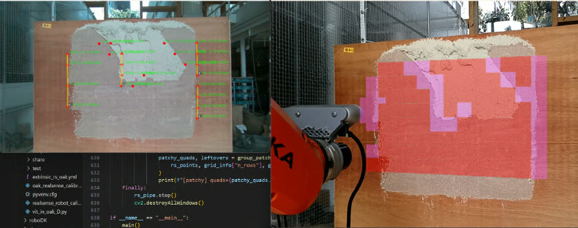
Around the model I built the things that made it usable. A tkinter annotation tool, because labeling 5,952 tiles through a file browser was not going to happen. A script that reconstructs a whole wall from predicted tiles in color, which is the figure at the top of this page and the fastest way to see that a model is wrong. And attention maps for each architecture, which is how I found that all of them latch onto the paint patch when there is one, and drift toward corners when a tile is uniform.

A colleague picked up the inference script and ran it on the arm before the end of my stay. It worked, and it also showed precision falling under real conditions, different lighting, occlusions, mud that had dried further than anything in my images. That gap is the one forty-two photographs predict, and it sits at the top of the recommendations I left for the next researcher, along with multiple annotators and a systematic ablation on the number of neighbors.

A robot arm facing a plastered wooden panel with the tile prediction overlay on it, next to a screen showing the inference script running. — The inference script on the arm, run by a colleague at the lab.

Read the paper, RCAE 2025, with Noborio, Muramoto and Du.